KL Sample Size Optimization

Introduction

Conditioned Latin hypercube sampling (cLHS) is widely used to select environmentally representative sampling locations, but it leaves one question open: how many samples are enough? Too few samples fail to represent the environmental variability of the study area; too many waste field and laboratory resources.

Malone et al. (2019) proposed answering this using Kullback-Leibler (KL) divergence: run cLHS at a range of candidate sample sizes, measure how well each sample’s distribution matches the population’s distribution across all covariates, and pick the smallest sample size that reaches a target level of representativeness.

This vignette walks through ss_kl_size() and its building blocks: ss_load_rasters(), ss_kl_divergence(), ss_kl_optimize(), and ss_kl_save_plots().

Theoretical Background

KL Divergence Between Population and Sample

For each numeric covariate, both the population and a candidate sample are binned into histograms over the same breaks. The KL divergence for that variable is:

$KL = \sum_i O_i \log\left(\frac{O_i}{E_i}\right)$

where $O_i$ is the sample’s density in bin $i$ and $E_i$ is the population’s density in the same bin. ss_kl_divergence() averages this across all numeric covariates, giving a single divergence score per sample: lower is better (more representative).

From Divergence to Optimal Sample Size

ss_kl_optimize() repeats this at a sequence of sample sizes (min_samples to max_samples, in step_size increments), running n_replicates independent cLHS draws at each size. The mean KL divergence per size is then fit to an exponential decay curve:

$KL(n) = b_1 e^{-kn} + b_0$

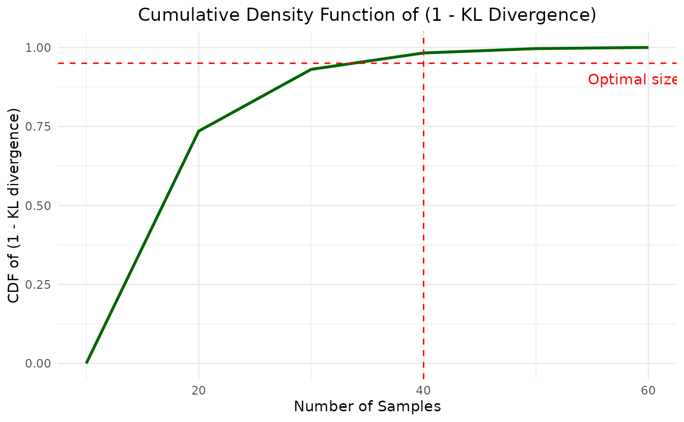
The optimal sample size is the smallest $n$ for which the cumulative proportion of achievable improvement,

$\frac{\max(KL) - KL(n)}{\max(KL) - \min(KL)},$

reaches probability_threshold (default 0.95) — i.e. the point of diminishing returns.

Basic Usage

ss_kl_size() accepts a raster path, an already-loaded SpatRaster, or a plain population data frame. For this vignette we build a small synthetic covariate stack so the example runs quickly and needs no external files.

library(soilsampling)
library(terra)

set.seed(42)

nr <- 40
nc <- 40

# Synthetic terrain-like covariates with spatial structure + noise
r <- rast(nrows = nr, ncols = nc, xmin = 0, xmax = 100, ymin = 0, ymax = 100, nlyrs = 3)
names(r) <- c("dem", "slope", "ndvi")

xy <- xyFromCell(r, seq_len(ncell(r)))
values(r)[, "dem"] <- 100 + 20 * sin(xy[, 1] / 15) + rnorm(ncell(r), 0, 3)
#> Warning: [readValues] raster has no values
values(r)[, "slope"] <- abs(cos(xy[, 2] / 12) * 8 + rnorm(ncell(r), 0, 1))
values(r)[, "ndvi"] <- pmin(pmax(0.5 + 0.3 * cos(xy[, 1] / 20 + xy[, 2] / 25) +
  rnorm(ncell(r), 0, 0.05), -1), 1)

r
#> class       : SpatRaster
#> size        : 40, 40, 3  (nrow, ncol, nlyr)
#> resolution  : 2.5, 2.5  (x, y)
#> extent      : 0, 100, 0, 100  (xmin, xmax, ymin, ymax)
#> coord. ref. : 
#> source(s)   : memory
#> names       :        dem,     slope,     ndvi
#> min values  :  71.914355,  0.007235, 0.057239
#> max values  : 127.422818, 10.770246, 0.958723

Running the End-to-End Workflow

result <- ss_kl_size(
  r,
  min_samples = 10,
  max_samples = 60,
  step_size = 10,
  n_replicates = 3,
  n_bins = 15
)

result$optimal_sample_size
#> [1] 40
result$summary_results
#> # A tibble: 6 × 3
#>   sample_size mean_kl   sd_kl
#>         <dbl>   <dbl>   <dbl>
#> 1          10  0.450  0.126  
#> 2          20  0.131  0.0340 
#> 3          30  0.0991 0.00468
#> 4          40  0.0583 0.0104 
#> 5          50  0.0295 0.00221
#> 6          60  0.0268 0.00166

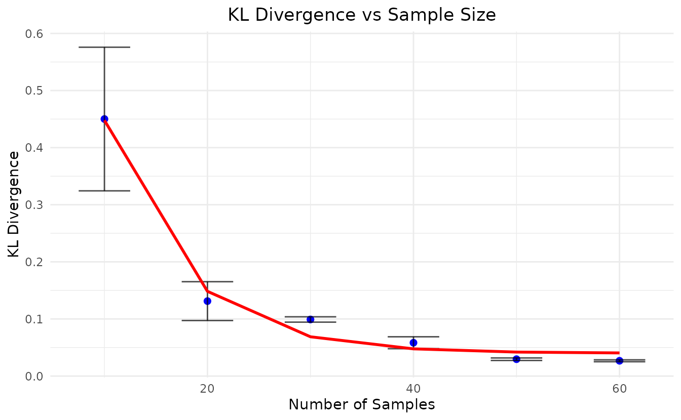
result$summary_results shows the mean and standard deviation of KL divergence at each tested sample size — you should see it decrease as sample size grows, then flatten out.

Visualizing the Result

result$plot_kl

result$plot_cdf

plot_kl shows the raw KL divergence values with the fitted exponential decay curve; plot_cdf shows the cumulative-improvement curve used to pick optimal_sample_size, with the threshold and chosen size marked.

Function Walkthrough

Loading Predictor Rasters

# Single multi-layer file
predictors <- ss_load_rasters("data/predictors.tif")

# Or a directory of single-layer .tif files
predictors <- ss_load_rasters("data/covariates/")

Computing KL Divergence Directly

If you already have a population and a candidate sample as data frames, you can skip the raster/cLHS machinery entirely:

population <- as.data.frame(r, na.rm = TRUE)
candidate_sample <- population[sample(nrow(population), 30), ]

ss_kl_divergence(population, candidate_sample, n_bins = 15)
#> [1] 0.2398814

Running the Optimizer on a Data Frame

ss_kl_optimize() is the engine behind ss_kl_size(). Use it directly when you already have a population data frame (e.g. from your own raster-to-data-frame pipeline):

opt <- ss_kl_optimize(
  population,
  min_samples = 10,
  max_samples = 60,
  step_size = 10,
  n_replicates = 3,
  n_bins = 15
)

opt$optimal_sample_size
#> [1] 30

Saving Plots Independently

ss_kl_size(..., output_dir = ...) writes CSVs and plots together. To save just the plots from a result you already have in memory (e.g. under a different naming scheme), use ss_kl_save_plots():

ss_kl_save_plots(result, output_dir = "my_outputs", prefix = "clhs_kl")

output_dir has no default: the function writes files, so the caller always chooses where they land.

Choosing Parameters

step_size: smaller steps give a finer-grained curve but multiply the number of cLHS runs. Start coarse (e.g. 20-50 for a few hundred candidate samples) and refine around the optimum if needed.
n_replicates: cLHS is stochastic, so each sample size needs multiple draws to estimate a stable mean KL divergence. 10 is a reasonable default for real analyses; this vignette uses 3 to keep runtime short.
n_bins: number of histogram bins per covariate. Too few bins blur real differences; too many make the divergence estimate noisy with small samples.
probability_threshold: how much of the achievable improvement you require before stopping. 0.95 (default) is a common choice; raise it if you can afford a larger sample, lower it if resources are tight.

Practical Workflow

library(soilsampling)

result <- ss_kl_size(
  "data/predictors.tif",
  min_samples = 10,
  max_samples = 500,
  step_size = 10,
  n_replicates = 10,
  probability_threshold = 0.95,
  output_dir = "outputs"
)

result$optimal_sample_size

# outputs/ now contains:
#   kl_raw_results.csv, kl_summary_results.csv, kl_fitted_curve.csv,
#   kl_divergence_vs_sample_size.png, kl_cdf_threshold.png

When to Use KL Sample Size Optimization

✅ Use it when:

You’re planning a cLHS design and need to justify the sample size
You want a data-driven stopping point instead of a fixed round number
Field/laboratory costs make oversampling expensive

❌ Don’t rely on it when:

Your sample size is fixed by budget or logistics regardless of the analysis
You have fewer than ~4 candidate sample sizes to test (the exponential fit needs more points to converge)

References

Malone, B.P., Minasny, B., and Brungard, C. (2019). Some methods to improve the utility of conditioned Latin hypercube sampling. PeerJ 7, e6451. DOI: 10.7717/peerj.6451
Minasny, B., and McBratney, A.B. (2006). A conditioned Latin hypercube method for sampling in the presence of ancillary information. Computers & Geosciences 32(9), 1378-1388. DOI: 10.1016/j.cageo.2005.12.009
Saurette, D.D., Heck, R.J., Gillespie, A.W., Berg, A.A., and Biswas, A. (2023). Divergence metrics for determining optimal training sample size in digital soil mapping. Geoderma 436, 116553. DOI: 10.1016/j.geoderma.2023.116553

soilsampling Package Authors

2026-08-02