Spatial Coverage Sampling Methods

Introduction

Spatial coverage sampling aims to provide optimal spatial distribution of sampling points across a study area. The soilsampling package implements spatial coverage using k-means clustering to create compact geographical strata, with samples placed at stratum centroids.

This approach is particularly effective for:

Model-based inference: Kriging and spatial interpolation
Soil mapping: Creating detailed soil maps
Environmental monitoring: Capturing spatial variability
Resource assessment: Estimating spatial distributions

Theoretical Background

The spatial coverage method is based on:

K-means clustering in geographic space to create compact strata
Stratification that minimizes Mean Squared Shortest Distance (MSSD)
Centroid sampling for optimal spatial coverage

The k-means algorithm partitions the study area into compact spatial strata by minimizing:

$\text{MSSD} = \frac{1}{m}\sum_{i=1}^{m} \min_k d^2(x_i, c_k)$

where $x_i$ are grid cell centers, $c_k$ are stratum centroids, and $d$ is Euclidean distance (or haversine distance for lat/lon coordinates).

Basic Usage

library(soilsampling)
library(sf)

# Create a study area
poly <- st_polygon(list(rbind(
  c(0, 0), c(100, 0), c(100, 50), c(0, 50), c(0, 0)
)))
study_area <- st_sf(geometry = st_sfc(poly))

# Set seed for reproducibility
set.seed(123)

Direct Coverage Sampling

# Create 25 coverage samples in one step
samples <- ss_coverage(study_area, n_strata = 25, n_try = 5)

print(samples)
#> Spatial Coverage Sampling 
#> ========================= 
#> Number of samples: 25 
#> Number of strata: 25

Two-Step Approach

# Step 1: Create stratification
strata <- ss_stratify(study_area, n_strata = 25, n_try = 5)

print(strata)
#> Soil Sampling Stratification
#> ============================
#> Number of strata: 25 
#> Number of cells: 2485 
#> Cell size: 1.41 x 1.41 
#> MSSD: 42.7747 
#> Converged: TRUE 
#> Equal area: FALSE

# Step 2: Extract centroids as sampling points
samples <- ss_coverage(strata)

# Plot both strata and samples
ss_plot(strata, samples = samples)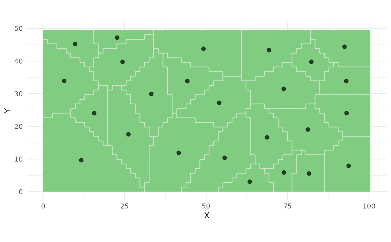

Algorithm Variants

The package implements two k-means variants:

1. Transfer Algorithm (Default)

Creates compact strata that may have unequal sizes:

# Standard spatial coverage
samples_transfer <- ss_coverage(study_area, n_strata = 20, n_try = 5)

# Check stratum sizes
strata_transfer <- ss_stratify(study_area, n_strata = 20, n_try = 5)
areas <- ss_relative_area(strata_transfer)
summary(areas)
#>    Min. 1st Qu.  Median    Mean 3rd Qu.    Max. 
#> 0.01730 0.02897 0.04547 0.05000 0.06539 0.09819

2. Swop Algorithm (Equal Area)

Creates strata of approximately equal size:

# Equal-area coverage sampling
samples_equal <- ss_coverage_equal_area(study_area, n_strata = 20, n_try = 5)

# Check stratum sizes
strata_equal <- ss_stratify(
  study_area,
  n_strata = 20,
  n_try = 5,
  equal_area = TRUE
)
areas_equal <- ss_relative_area(strata_equal)
summary(areas_equal)
#>    Min. 1st Qu.  Median    Mean 3rd Qu.    Max. 
#>  0.0499  0.0499  0.0499  0.0500  0.0500  0.0503

The equal-area variant is particularly useful for composite sampling where you need equal representation from each stratum.

Incorporating Prior Points

You can incorporate existing sampling locations as fixed stratum centers:

# Suppose we have 2 existing sampling locations
prior_pts <- st_as_sf(
  data.frame(x = c(25, 75), y = c(25, 25)),
  coords = c("x", "y")
)

# Create stratification with prior points
strata_prior <- ss_stratify(
  study_area,
  n_strata = 20,
  prior_points = prior_pts,
  n_try = 5
)

# Get coverage samples
samples_prior <- ss_coverage(strata_prior)

# Plot with prior points highlighted
ss_plot(samples_prior)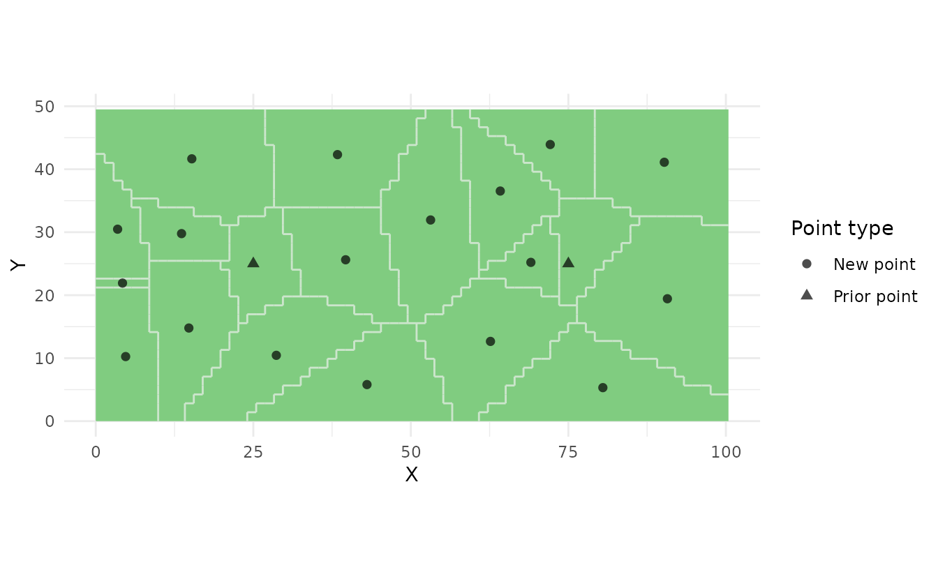

Prior points are useful when: - Adding to an existing monitoring network - Incorporating legacy sampling locations - Designing adaptive sampling schemes

Optimizing Parameters

Number of Strata

The choice of n_strata depends on:

Survey budget: More strata = more samples
Spatial variability: More heterogeneous areas need more samples
Mapping resolution: Finer maps need more samples

# Compare different numbers of strata
samples_10 <- ss_coverage(study_area, n_strata = 10, n_try = 5)
samples_50 <- ss_coverage(study_area, n_strata = 50, n_try = 5)

par(mfrow = c(1, 2))
plot(st_geometry(study_area), main = "10 strata")
plot(st_geometry(samples_10$samples), add = TRUE, pch = 19, col = "red")

plot(st_geometry(study_area), main = "50 strata")
plot(st_geometry(samples_50$samples), add = TRUE, pch = 19, col = "red")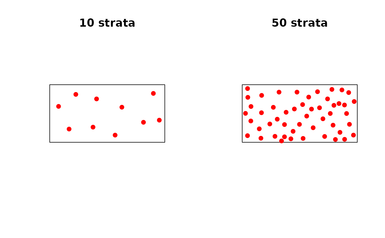

par(mfrow = c(1, 1))

Number of Tries

The n_try parameter controls how many random initializations to use:

# Compare convergence with different n_try values
set.seed(456)
result_1 <- ss_stratify(study_area, n_strata = 25, n_try = 1)
result_5 <- ss_stratify(study_area, n_strata = 25, n_try = 5)
result_20 <- ss_stratify(study_area, n_strata = 25, n_try = 20)

cat("n_try = 1:  MSSD =", format(result_1$mssd, digits = 6), "\n")
#> n_try = 1:  MSSD = 44.7988
cat("n_try = 5:  MSSD =", format(result_5$mssd, digits = 6), "\n")
#> n_try = 5:  MSSD = 42.2537
cat("n_try = 20: MSSD =", format(result_20$mssd, digits = 6), "\n")
#> n_try = 20: MSSD = 40.4673

Higher n_try generally produces better results but takes longer.

Grid Resolution

Control discretization resolution with n_cells or cell_size:

# Coarse grid (fast)
strata_coarse <- ss_stratify(
  study_area,
  n_strata = 25,
  n_cells = 500,
  n_try = 3
)

# Fine grid (slower but more precise)
strata_fine <- ss_stratify(
  study_area,
  n_strata = 25,
  n_cells = 5000,
  n_try = 3
)

cat("Coarse grid:", nrow(strata_coarse$cells), "cells\n")
#> Coarse grid: 512 cells
cat("Fine grid:  ", nrow(strata_fine$cells), "cells\n")
#> Fine grid:   5000 cells

Stratified Random Sampling

For design-based inference, use stratified random sampling instead of centroid placement:

# Create strata
strata <- ss_stratify(study_area, n_strata = 25, n_try = 5)

# Take 1 random sample per stratum
samples_strat <- ss_stratified(strata, n_per_stratum = 1)

# Or take multiple samples per stratum
samples_strat_3 <- ss_stratified(strata, n_per_stratum = 3)

ss_plot(strata, samples = samples_strat_3)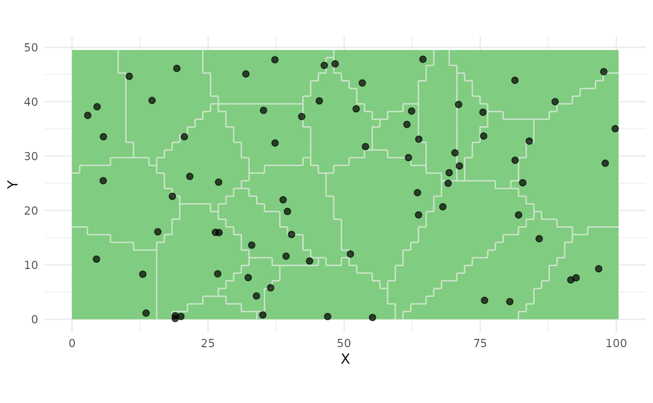

This provides: - Valid probability sampling - Unbiased estimates of means and totals - Better precision than simple random sampling

Composite Sampling

For laboratory cost reduction, combine samples from multiple locations:

# Create 3 composite samples from 20 equal-area strata
samples_comp <- ss_composite(study_area, n_strata = 20, n_composites = 3)

# Each composite includes one sample from each stratum
ss_plot(samples_comp)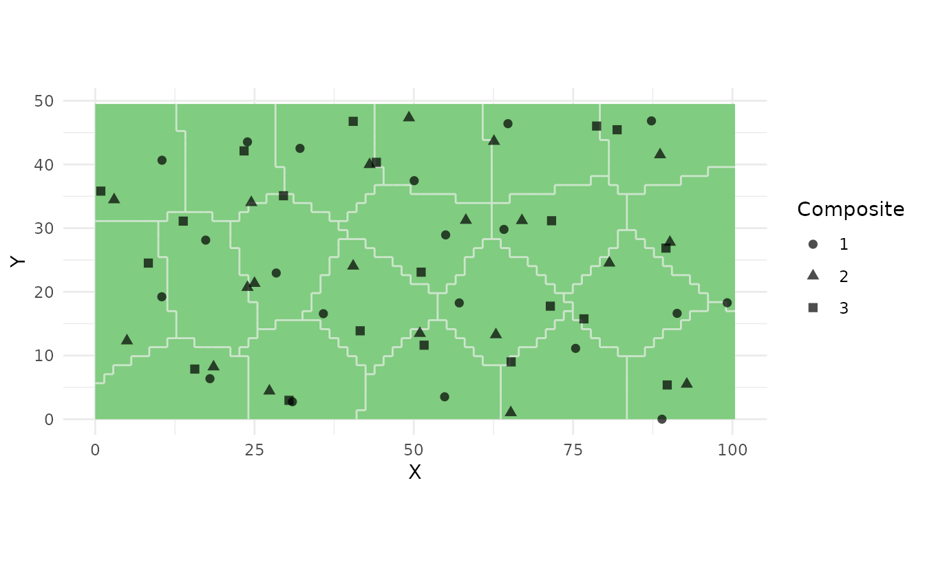

Working with Geographic Coordinates

The package handles lat/lon coordinates automatically:

# Study area with geographic CRS
study_area_geo <- st_transform(study_area, crs = 4326)

# The algorithm uses haversine distance automatically
samples_geo <- ss_coverage(study_area_geo, n_strata = 25, n_try = 5)

# Note: equal_area is not supported for lat/lon
# This will produce an error:
# samples_error <- ss_coverage_equal_area(study_area_geo, n_strata = 25)

Practical Workflow

A typical workflow for a soil survey:

# 1. Load study area
study_area <- st_read("my_field.shp")

# 2. Design sampling scheme
set.seed(42)  # For reproducibility
samples <- ss_coverage(study_area, n_strata = 50, n_try = 10)

# 3. Examine results
print(samples)
summary(samples)

# 4. Export for field work
coords <- ss_to_data_frame(samples)
write.csv(coords, "field_sampling_locations.csv", row.names = FALSE)

# 5. Export as shapefile for GPS
st_write(ss_to_sf(samples), "sampling_points.gpkg")

Comparison with Other Methods

set.seed(789)

# Spatial coverage
samp_coverage <- ss_coverage(study_area, n_strata = 25, n_try = 5)

# Stratified random
strata <- ss_stratify(study_area, n_strata = 25, n_try = 5)
samp_stratified <- ss_stratified(strata, n_per_stratum = 1)

# Simple random
samp_random <- ss_random(study_area, n = 25)

# Compare spatial distribution
par(mfrow = c(1, 3))

plot(st_geometry(study_area), main = "Coverage")
plot(st_geometry(samp_coverage$samples), add = TRUE, pch = 19, col = "red")

plot(st_geometry(study_area), main = "Stratified Random")
plot(st_geometry(samp_stratified$samples), add = TRUE, pch = 19, col = "blue")

plot(st_geometry(study_area), main = "Simple Random")
plot(st_geometry(samp_random$samples), add = TRUE, pch = 19, col = "green")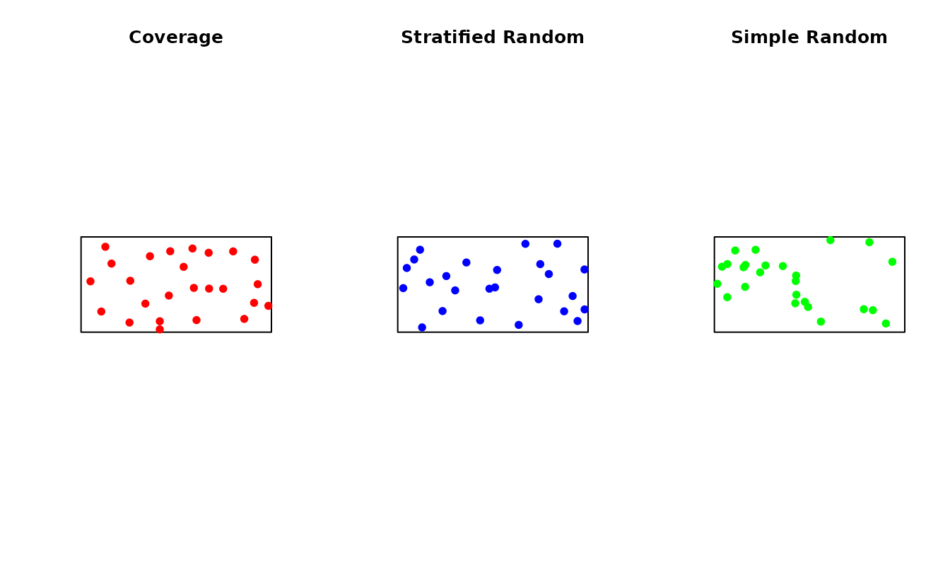


par(mfrow = c(1, 1))

References

Walvoort, D.J.J., Brus, D.J., and de Gruijter, J.J. (2010). An R package for spatial coverage sampling and random sampling from compact geographical strata by k-means. Computers & Geosciences 36, 1261-1267. DOI: 10.1016/j.cageo.2010.04.005
de Gruijter, J.J., Brus, D.J., Bierkens, M.F.P., and Knotters, M. (2006). Sampling for Natural Resource Monitoring. Springer, Berlin.
Brus, D.J. and de Gruijter, J.J. (1997). Random sampling or geostatistical modelling? Choosing between design-based and model-based sampling strategies for soil. Geoderma 80(1-2), 1-44.

soilsampling Package Authors

2025-12-26