Introduction to soilsampling

Overview

The soilsampling package provides methods for designing soil sampling schemes, including:

Simple Random Sampling: Uniform random selection of sampling locations
Stratified Random Sampling: Random sampling within compact geographical strata
Spatial Coverage Sampling: Purposive sampling at stratum centroids for optimal coverage
Maxvol Optimal Design: D-optimal design using maximum volume criterion
Composite Sampling: Sampling from equal-area strata for combined samples

The package uses sf for spatial operations and implements pure R algorithms, requiring no Java or additional GIS software.

Installation

# Install from local source
install.packages(".", repos = NULL, type = "source")

# Or using devtools
devtools::install()

Quick Start

library(soilsampling)
library(sf)

# Create a study area
poly <- st_polygon(list(rbind(
  c(0, 0), c(100, 0), c(100, 50), c(0, 50), c(0, 0)
)))
study_area <- st_sf(geometry = st_sfc(poly))

Spatial Coverage Sampling

# Set seed for reproducibility
set.seed(42)

# Create spatial coverage sampling design
samples_coverage <- ss_coverage(study_area, n_strata = 25, n_try = 5)

# View summary
print(samples_coverage)
#> Spatial Coverage Sampling 
#> ========================= 
#> Number of samples: 25 
#> Number of strata: 25

# Plot
ss_plot(samples_coverage)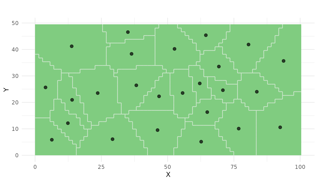

Stratified Random Sampling

# First create strata
strata <- ss_stratify(study_area, n_strata = 25, n_try = 5)

# Take random samples within each stratum
samples_stratified <- ss_stratified(strata, n_per_stratum = 1)

# Plot
ss_plot(strata, samples = samples_stratified)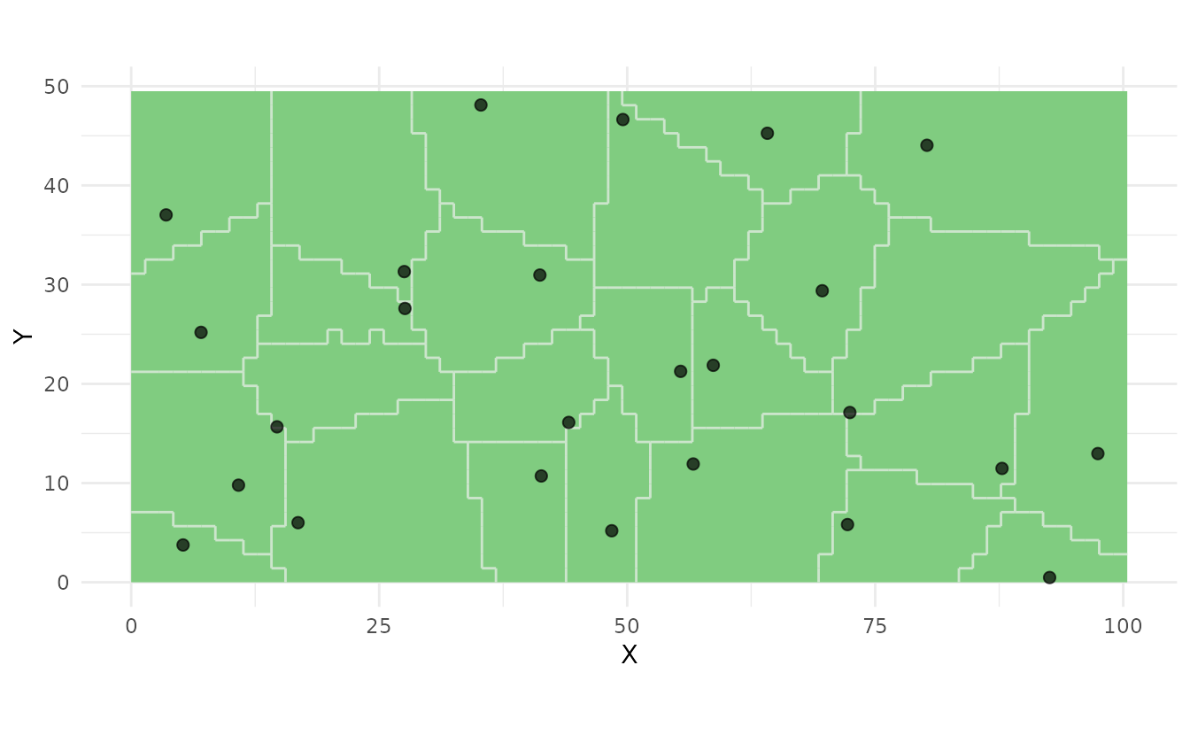

Simple Random Sampling

# Simple random sampling
samples_random <- ss_random(study_area, n = 25)

# Plot
ss_plot_samples(samples_random)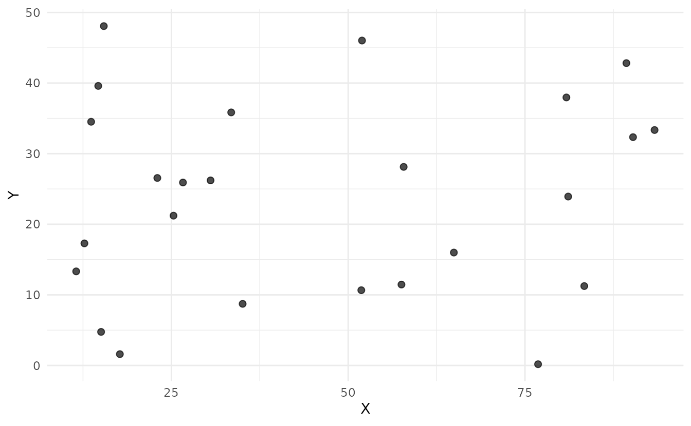

Exporting Results

As Data Frame

# Get coordinates as data frame
coords <- ss_to_data_frame(samples_coverage)
head(coords)
#>   sample_id stratum_id is_prior        X        Y
#> 1         1          1    FALSE 35.02039 46.55740
#> 2         2          2    FALSE 55.66225 23.53371
#> 3         3          3    FALSE 46.77691 22.27986
#> 4         4          4    FALSE 62.12984 27.15672
#> 5         5          5    FALSE 92.47119 10.56665
#> 6         6          6    FALSE 52.60995 40.20839

As CSV

# Export to CSV
write.csv(coords, "sampling_points.csv", row.names = FALSE)

As Shapefile or GeoPackage

# Get as sf object
samples_sf <- ss_to_sf(samples_coverage)

# Export to GeoPackage
st_write(samples_sf, "sampling_points.gpkg")

# Export to Shapefile
st_write(samples_sf, "sampling_points.shp")

Working with Real Data

In practice, you would load a study area from a shapefile:

# Read study area from shapefile
study_area <- st_read("path/to/study_area.shp")

# Create sampling design
set.seed(42)
samples <- ss_coverage(study_area, n_strata = 50, n_try = 10)

# Export coordinates
coords <- ss_to_data_frame(samples)
write.csv(coords, "field_sampling_points.csv", row.names = FALSE)

When to Use Each Method

Method	Best For	Inference Type	Key Features
`ss_coverage()`	Interpolation (kriging)	Model-based	Optimal spatial coverage
`ss_stratified()`	Estimating means/totals	Design-based	Valid probability sample
`ss_random()`	Simple design-based analysis	Design-based	Unbiased estimates
`ss_maxvol()`	Optimal feature coverage	Model-based	D-optimal design
`ss_composite()`	Reducing laboratory costs	Design-based	Combined samples

Sampling Methods Comparison

Design-Based vs Model-Based

Design-based sampling (e.g., ss_random(), ss_stratified()): - Uses probability sampling - Statistical inference based on sampling design - Valid for design-based estimation (means, totals) - No assumptions about spatial autocorrelation required

Model-based sampling (e.g., ss_coverage(), ss_maxvol()): - Purposive (non-random) sample selection - Requires spatial model for inference (e.g., kriging) - Optimal for prediction and interpolation - More efficient for mapping applications

Tips for Best Results

Use multiple tries: Set n_try = 10 or higher to avoid local optima in k-means algorithms
Set a seed: Use set.seed() for reproducible results
Adjust resolution: Use n_cells parameter to control grid density
Check convergence: The output includes a converged flag
Consider prior information: Use prior_points to incorporate existing sample locations

Getting Help

For more detailed information on specific methods, see:

vignette("spatial-coverage") - Spatial coverage sampling methods
vignette("maxvol-sampling") - Maxvol optimal design sampling
?ss_stratify - Help on stratification
?ss_coverage - Help on coverage sampling
?ss_maxvol - Help on maxvol sampling

References

de Gruijter, J.J., Brus, D.J., Bierkens, M.F.P., and Knotters, M. (2006). Sampling for Natural Resource Monitoring. Springer, Berlin.
Walvoort, D.J.J., Brus, D.J., and de Gruijter, J.J. (2010). An R package for spatial coverage sampling and random sampling from compact geographical strata by k-means. Computers & Geosciences 36, 1261-1267.
Petrovskaia, A., Ryzhakov, G., & Oseledets, I. (2021). Optimal soil sampling design based on the maxvol algorithm. Geoderma, 383, 114733.

soilsampling Package Authors

2025-12-26