cLHS + Random Forest Optimization

Introduction

Conditioned Latin hypercube sampling (cLHS) gives a design that is environmentally representative, but representativeness is not the same as predictive accuracy. Wadoux et al. (2019) showed that a cLHS baseline can be further improved for a specific prediction task by directly optimizing the sample locations against a Random Forest’s cross-validated prediction error.

This package implements that idea as a two-stage workflow:

cLHS baseline: generate a representative starting design (ss_clhs_sample())
Simulated annealing refinement: iteratively swap sample points to minimize Random Forest MSE (ss_rf_optimize())

ss_rf_size() runs both stages end-to-end and produces comparison plots.

Theoretical Background

The Objective Function

At each candidate design, ss_rf_mse() fits a Random Forest with $k$ -fold cross-validation, predicting one covariate (the “response”) from the others, and returns the mean squared error averaged across folds. Lower MSE means the design’s points are more informative for predicting that variable from the rest.

Simulated Annealing

ss_rf_optimize() starts from the cLHS baseline and repeats, for n_iterations:

Replace one randomly chosen sample point with a randomly chosen point not currently in the design
Compute the candidate design’s RF MSE
Accept the swap if it improves MSE, or probabilistically accept a worse swap with probability $\exp(-\Delta / T)$ (the Metropolis criterion)
Cool the temperature: $T \leftarrow T \times \text{cooling\_rate}$

Early iterations (high temperature) tolerate worse moves, allowing the search to escape local optima; later iterations (low temperature) only accept improvements, converging to a refined design. The best design seen at any point is tracked and returned, regardless of where the search ends up.

Basic Usage

As in the KL sample size vignette, we build a small synthetic covariate stack so the example runs quickly.

library(soilsampling)
library(terra)

set.seed(7)

nr <- 30
nc <- 30

r <- rast(nrows = nr, ncols = nc, xmin = 0, xmax = 100, ymin = 0, ymax = 100, nlyrs = 3)
names(r) <- c("dem", "slope", "ndvi")

xy <- xyFromCell(r, seq_len(ncell(r)))
values(r)[, "dem"] <- 100 + 20 * sin(xy[, 1] / 15) + rnorm(ncell(r), 0, 3)
#> Warning: [readValues] raster has no values
values(r)[, "slope"] <- abs(cos(xy[, 2] / 12) * 8 + rnorm(ncell(r), 0, 1))
values(r)[, "ndvi"] <- pmin(pmax(0.5 + 0.3 * cos(xy[, 1] / 20 + xy[, 2] / 25) +
  rnorm(ncell(r), 0, 0.05), -1), 1)

r
#> class       : SpatRaster
#> size        : 30, 30, 3  (nrow, ncol, nlyr)
#> resolution  : 3.333333, 3.333333  (x, y)
#> extent      : 0, 100, 0, 100  (xmin, xmax, ymin, ymax)
#> coord. ref. : 
#> source(s)   : memory
#> names       :        dem,     slope,     ndvi
#> min values  :  72.751228,   0.00331, 0.062757
#> max values  : 126.185615, 11.297571, 0.937295

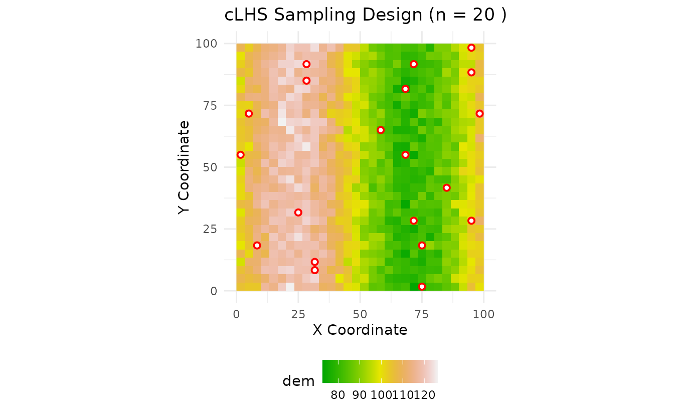
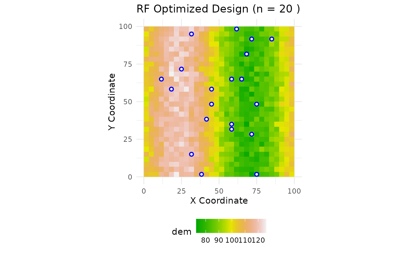
Running the End-to-End Workflow

result <- ss_rf_size(
  r,
  n_samples = 20,
  n_iterations = 30,
  seed = 123
)

result$comparison_table
#>         Method    MSE Samples Improvement
#> 1         cLHS 0.0506      20         0.0
#> 2 RF Optimized 0.0254      20        49.8
result$improvement
#> [1] 49.79946

result$improvement is the percent reduction in cross-validated MSE achieved by the RF-optimized design relative to the cLHS baseline.

Visualizing the Comparison

result$plots$clhs_plot

result$plots$rf_plot

Function Walkthrough

cLHS Baseline Alone

baseline <- ss_clhs_sample(r, n_samples = 20, seed = 123)
head(baseline)
#>             x         y       dem     slope      ndvi
#> 893 75.000000  1.666667  75.39868 9.2237535 0.2489234
#> 723  8.333333 18.333333 111.31117 0.4359382 0.6828071
#> 242  5.000000 71.666667 107.00959 6.3445575 0.1700880
#> 391  1.666667 55.000000 100.01737 0.6546141 0.3312138
#> 652 71.666667 28.333333  85.73679 5.5000503 0.4925988
#> 69  28.333333 91.666667 122.77872 1.6802305 0.5888598

Evaluating a Design’s MSE Directly

ss_rf_mse(baseline)
#> [1] 0.05063079

By default, the third covariate column is used as the response (predicted from the rest); pass target_var to choose a different one.

ss_rf_mse(baseline, target_var = "ndvi")
#> [1] 0.04944906

Running the Optimizer on Its Own

opt <- ss_rf_optimize(
  r,
  n_samples = 20,
  n_iterations = 30,
  seed = 123
)

opt$initial_mse
#> [1] 0.05063079
opt$final_mse
#> [1] 0.02541693
opt$improvement
#> [1] 49.79946

Choosing Parameters

n_iterations: more iterations give the search more chances to improve, at a roughly linear cost in runtime (one RF fit per iteration). This vignette uses 30 to stay fast; real analyses typically use several hundred.
temperature / cooling_rate: higher initial temperature and slower cooling (cooling_rate closer to 1) explore more broadly before converging, at the cost of more iterations needed to settle. The defaults (1000 / 0.95) work well for designs of a few dozen to a few hundred points.
target_var: choose the covariate that best represents your actual prediction target (e.g. an observed soil property in real data), not necessarily the default third column.
seed: the cLHS baseline uses seed; the annealing loop uses seed + 1, so both stages are reproducible independently.

Practical Workflow

library(soilsampling)
library(terra)

predictors <- rast("data/predictors.tif")

result <- ss_rf_size(
  predictors,
  n_samples = 100,
  n_iterations = 500,
  seed = 123,
  output_dir = "outputs"
)

result$comparison_table
result$improvement

# outputs/ now contains:
#   clhs_sample_locations.csv, rf_optimized_locations.csv,
#   sampling_comparison_table.csv, sampling_comparison_plots.png

When to Use cLHS + RF Optimization

✅ Use it when:

You have a specific covariate (or measured property) you want to predict well, not just represent
A Random Forest (or similar model) is a realistic stand-in for your eventual prediction workflow
You can afford the extra computation of iterative RF fitting on top of cLHS

❌ Don’t rely on it when:

You need probability-based sampling for design-based (not model-based) inference
Your prediction target isn’t known yet, or differs substantially from the covariates used for optimization
The candidate pool is very large and RF fitting per iteration becomes prohibitively slow — consider a coarser candidate grid first

References

Wadoux, A.M.J-C., Brus, D.J., and Heuvelink, G.B.M. (2019). Sampling design optimization for soil mapping with random forest. Geoderma 355, 113913. DOI: 10.1016/j.geoderma.2019.113913
Minasny, B., and McBratney, A.B. (2006). A conditioned Latin hypercube method for sampling in the presence of ancillary information. Computers & Geosciences 32(9), 1378-1388. DOI: 10.1016/j.cageo.2005.12.009
Breiman, L. (2001). Random forests. Machine Learning 45(1), 5-32. DOI: 10.1023/A:1010933404324
Kirkpatrick, S., Gelatt, C.D., and Vecchi, M.P. (1983). Optimization by simulated annealing. Science 220(4598), 671-680. DOI: 10.1126/science.220.4598.671

soilsampling Package Authors

2026-08-02