Introduction to soilquality

Overview

The soilquality package provides tools for calculating Soil Quality Index (SQI) using a scientifically rigorous approach that combines:

Principal Component Analysis (PCA) for selecting a Minimum Data Set (MDS) of soil indicators
Analytic Hierarchy Process (AHP) for expert-based weighting of indicators
Flexible scoring functions for normalizing soil properties to a 0-1 scale
Visualization tools for interpreting and communicating results

This package is designed for soil scientists, researchers, and environmental consultants who need to assess soil quality in a systematic and reproducible way.

Installation

From GitHub

You can install the development version of soilquality from GitHub:

# Install devtools if you haven't already
install.packages("devtools")

# Install soilquality from GitHub
devtools::install_github("username/soilquality")

From CRAN

Once released on CRAN, you can install the package with:

install.packages("soilquality")

Basic Workflow

The typical workflow for calculating SQI involves these steps:

Load and prepare your soil data
Select soil properties for analysis
Define scoring rules for each property
Calculate indicator weights (optional: use AHP)
Compute the SQI
Visualize and interpret results

Let’s walk through a complete example using the included soil_ucayali dataset.

Load the Package and Data

library(soilquality)

# Load the example dataset
data(soil_ucayali)

# View the first few rows
head(soil_ucayali)
#>   SampleID Sand Silt Clay   BD  pH   OM  SOC     N    P   K  CEC   Ca   Mg   EC
#> 1   UCY001 42.4 35.4 22.2 1.47 7.0 2.46 1.24 0.201  7.8 131 10.2 5.51 2.44 0.06
#> 2   UCY002 42.7 30.2 27.1 1.47 6.2 2.29 1.22 0.050  4.5 121  9.0 3.56 1.78 0.26
#> 3   UCY003 54.6 25.4 20.0 1.40 5.0 2.49 1.13 0.129  6.1 106 15.1 5.83 1.78 0.31
#> 4   UCY004 41.9 37.4 20.7 1.20 5.6 2.88 1.07 0.156  7.9 113 14.3 4.80 0.89 0.10
#> 5   UCY005 50.1 30.3 19.6 1.33 4.9 4.24 1.38 0.105 10.0 118  7.5 6.48 2.27 0.30
#> 6   UCY006 49.5 31.8 18.7 1.31 4.8 2.72 1.77 0.167  3.0  40 11.7 2.75 1.67 0.17

The soil_ucayali dataset contains 50 soil samples from the Ucayali region of Peru, with 14 soil properties including physical, chemical, and fertility indicators.

Quick Start: Basic SQI Calculation

The simplest way to calculate SQI is using compute_sqi_properties() with default settings:

# Calculate SQI using standard fertility properties
result <- compute_sqi_properties(
  data = soil_ucayali,
  properties = c("pH", "OM", "N", "P", "K", "CEC"),
  id_column = "SampleID"
)

# View the result
print(result)
#> $mds
#> [1] "N"  "K"  "P"  "pH" "OM"
#> 
#> $weights
#>   N   K   P  pH  OM 
#> 0.2 0.2 0.2 0.2 0.2 
#> 
#> $CR
#> [1] 0
#> 
#> $results
#>    SampleID  pH   OM     N    P   K  CEC   N_scored  K_scored   P_scored
#> 1    UCY001 7.0 2.46 0.201  7.8 131 10.2 0.65938865 0.8750000 0.43939394
#> 2    UCY002 6.2 2.29 0.050  4.5 121  9.0 0.00000000 0.7788462 0.18939394
#> 3    UCY003 5.0 2.49 0.129  6.1 106 15.1 0.34497817 0.6346154 0.31060606
#> 4    UCY004 5.6 2.88 0.156  7.9 113 14.3 0.46288210 0.7019231 0.44696970
#> 5    UCY005 4.9 4.24 0.105 10.0 118  7.5 0.24017467 0.7500000 0.60606061
#> 6    UCY006 4.8 2.72 0.167  3.0  40 11.7 0.51091703 0.0000000 0.07575758
#> 7    UCY007 4.6 3.77 0.171  7.0 123  9.3 0.52838428 0.7980769 0.37878788
#> 8    UCY008 4.7 3.37 0.148 10.3  83  5.8 0.42794760 0.4134615 0.62878788
#> 9    UCY009 6.5 2.70 0.050  6.4 101 12.5 0.00000000 0.5865385 0.33333333
#> 10   UCY010 5.2 1.42 0.279  8.7  88 11.8 1.00000000 0.4615385 0.50757576
#> 11   UCY011 5.3 2.33 0.140  9.5 117 11.7 0.39301310 0.7403846 0.56818182
#> 12   UCY012 5.4 2.36 0.183  8.8  86 12.6 0.58078603 0.4423077 0.51515152
#> 13   UCY013 6.2 2.84 0.164 10.0 108 14.6 0.49781659 0.6538462 0.60606061
#> 14   UCY014 4.8 3.97 0.201  7.6  85 12.6 0.65938865 0.4326923 0.42424242
#> 15   UCY015 4.4 4.86 0.191  6.8  68 10.2 0.61572052 0.2692308 0.36363636
#> 16   UCY016 6.5 4.19 0.140  2.0 125  9.8 0.39301310 0.8173077 0.00000000
#> 17   UCY017 4.8 2.68 0.169  7.7 114 11.6 0.51965066 0.7115385 0.43181818
#> 18   UCY018 4.6 1.22 0.103  9.3 138 12.9 0.23144105 0.9423077 0.55303030
#> 19   UCY019 4.2 2.45 0.193  9.6  97  8.9 0.62445415 0.5480769 0.57575758
#> 20   UCY020 4.2 2.88 0.127  6.3 123 11.4 0.33624454 0.7980769 0.32575758
#> 21   UCY021 4.7 3.56 0.271 13.3 144 14.9 0.96506550 1.0000000 0.85606061
#> 22   UCY022 5.7 3.67 0.067  8.9  88 11.7 0.07423581 0.4615385 0.52272727
#> 23   UCY023 6.1 3.42 0.127  8.4  62  9.9 0.33624454 0.2115385 0.48484848
#> 24   UCY024 5.8 1.54 0.191 11.8  89 11.2 0.61572052 0.4711538 0.74242424
#> 25   UCY025 4.9 3.56 0.176  5.8  90 15.3 0.55021834 0.4807692 0.28787879
#> 26   UCY026 5.2 2.40 0.121  6.6  99 13.7 0.31004367 0.5673077 0.34848485
#> 27   UCY027 4.6 2.96 0.100 15.2 138 15.7 0.21834061 0.9423077 1.00000000
#> 28   UCY028 4.6 2.87 0.157  8.0  87 12.4 0.46724891 0.4519231 0.45454545
#> 29   UCY029 5.9 3.19 0.149 12.9 104 13.2 0.43231441 0.6153846 0.82575758
#> 30   UCY030 4.4 2.82 0.060  3.7  89 10.3 0.04366812 0.4711538 0.12878788
#> 31   UCY031 6.8 1.30 0.152  7.4  96 13.8 0.44541485 0.5384615 0.40909091
#> 32   UCY032 5.1 3.46 0.160  9.1 103 10.5 0.48034934 0.6057692 0.53787879
#> 33   UCY033 5.4 3.15 0.159  8.9 128  7.7 0.47598253 0.8461538 0.52272727
#> 34   UCY034 4.6 2.56 0.097  5.0  98 12.4 0.20524017 0.5576923 0.22727273
#> 35   UCY035 4.7 2.91 0.174  8.1 113 17.8 0.54148472 0.7019231 0.46212121
#> 36   UCY036 4.1 2.92 0.219  4.8 114 14.4 0.73799127 0.7115385 0.21212121
#> 37   UCY037 5.1 3.00 0.173 10.1 118 15.5 0.53711790 0.7500000 0.61363636
#> 38   UCY038 5.5 4.28 0.093 11.3  81 13.1 0.18777293 0.3942308 0.70454545
#> 39   UCY039 5.5 2.60 0.128  2.0 136 10.2 0.34061135 0.9230769 0.00000000
#> 40   UCY040 4.6 2.95 0.167 11.7  85 11.4 0.51091703 0.4326923 0.73484848
#> 41   UCY041 4.6 3.85 0.118  4.3  92 11.2 0.29694323 0.5000000 0.17424242
#> 42   UCY042 4.8 3.75 0.050  9.4 130 10.6 0.00000000 0.8653846 0.56060606
#> 43   UCY043 6.4 3.83 0.194 10.0 127 14.1 0.62882096 0.8365385 0.60606061
#> 44   UCY044 4.3 2.28 0.109  7.4  68  8.4 0.25764192 0.2692308 0.40909091
#> 45   UCY045 5.1 4.60 0.121  6.1  73 14.6 0.31004367 0.3173077 0.31060606
#> 46   UCY046 6.7 2.86 0.225  8.5  61 14.6 0.76419214 0.2019231 0.49242424
#> 47   UCY047 5.1 4.48 0.111  9.3 100  8.4 0.26637555 0.5769231 0.55303030
#> 48   UCY048 4.1 1.58 0.192 10.6  99 13.9 0.62008734 0.5673077 0.65151515
#> 49   UCY049 4.7 2.82 0.087  2.0 104 19.3 0.16157205 0.6153846 0.00000000
#> 50   UCY050 5.6 3.92 0.132  3.1 109 10.3 0.35807860 0.6634615 0.08333333
#>     pH_scored  OM_scored       SQI
#> 1  1.00000000 0.34065934 0.6628884
#> 2  0.72413793 0.29395604 0.3972668
#> 3  0.31034483 0.34890110 0.3898891
#> 4  0.51724138 0.45604396 0.5170120
#> 5  0.27586207 0.82967033 0.5403535
#> 6  0.24137931 0.41208791 0.2480284
#> 7  0.17241379 0.70054945 0.5156425
#> 8  0.20689655 0.59065934 0.4535506
#> 9  0.82758621 0.40659341 0.4308103
#> 10 0.37931034 0.05494505 0.4806739
#> 11 0.41379310 0.30494505 0.4840635
#> 12 0.44827586 0.31318681 0.4599416
#> 13 0.72413793 0.44505495 0.5853832
#> 14 0.24137931 0.75549451 0.5026394
#> 15 0.10344828 1.00000000 0.4704072
#> 16 0.82758621 0.81593407 0.5707682
#> 17 0.24137931 0.40109890 0.4610971
#> 18 0.17241379 0.00000000 0.3798386
#> 19 0.03448276 0.33791209 0.4241367
#> 20 0.03448276 0.45604396 0.3901212
#> 21 0.20689655 0.64285714 0.7341760
#> 22 0.55172414 0.67307692 0.4566605
#> 23 0.68965517 0.60439560 0.4653365
#> 24 0.58620690 0.08791209 0.5006835
#> 25 0.27586207 0.64285714 0.4475171
#> 26 0.37931034 0.32417582 0.3858645
#> 27 0.17241379 0.47802198 0.5622168
#> 28 0.17241379 0.45329670 0.3998856
#> 29 0.62068966 0.54120879 0.6070710
#> 30 0.10344828 0.43956044 0.2373237
#> 31 0.93103448 0.02197802 0.4691960
#> 32 0.34482759 0.61538462 0.5168419
#> 33 0.44827586 0.53021978 0.5646719
#> 34 0.17241379 0.36813187 0.3061502
#> 35 0.20689655 0.46428571 0.4753423
#> 36 0.00000000 0.46703297 0.4257368
#> 37 0.34482759 0.48901099 0.5469186
#> 38 0.48275862 0.84065934 0.5219934
#> 39 0.48275862 0.37912088 0.4251136
#> 40 0.17241379 0.47527473 0.4652293
#> 41 0.17241379 0.72252747 0.3732254
#> 42 0.24137931 0.69505495 0.4724850
#> 43 0.79310345 0.71703297 0.7163113
#> 44 0.06896552 0.29120879 0.2592276
#> 45 0.34482759 0.92857143 0.4422713
#> 46 0.89655172 0.45054945 0.5611281
#> 47 0.34482759 0.89560440 0.5273522
#> 48 0.00000000 0.09890110 0.3875623
#> 49 0.20689655 0.43956044 0.2846827
#> 50 0.51724138 0.74175824 0.4727746
#> 
#> $pca
#> Standard deviations (1, .., p=6):
#> [1] 1.2017266 1.0469160 1.0156199 0.9785231 0.9083996 0.8035165
#> 
#> Rotation (n x k) = (6 x 6):
#>             PC1        PC2        PC3        PC4         PC5         PC6
#> pH  -0.04895981 -0.5700395  0.1154650 -0.7904182  0.18441227 -0.02359874
#> OM   0.44217933  0.2758787 -0.4027009 -0.1167926  0.73550006  0.10770122
#> N   -0.54756497  0.4423174  0.0590335 -0.2826793  0.05604688  0.64652461
#> P   -0.48824240  0.2012391 -0.5880626 -0.1952384 -0.05022056 -0.57850192
#> K   -0.23046074 -0.5905356 -0.5414652  0.3629924  0.06094813  0.41169512
#> CEC -0.45908625 -0.1186244  0.4266295  0.3343793  0.64471214 -0.25630475
#> 
#> $loadings
#>             PC1        PC2        PC3        PC4         PC5         PC6
#> pH  -0.04895981 -0.5700395  0.1154650 -0.7904182  0.18441227 -0.02359874
#> OM   0.44217933  0.2758787 -0.4027009 -0.1167926  0.73550006  0.10770122
#> N   -0.54756497  0.4423174  0.0590335 -0.2826793  0.05604688  0.64652461
#> P   -0.48824240  0.2012391 -0.5880626 -0.1952384 -0.05022056 -0.57850192
#> K   -0.23046074 -0.5905356 -0.5414652  0.3629924  0.06094813  0.41169512
#> CEC -0.45908625 -0.1186244  0.4266295  0.3343793  0.64471214 -0.25630475
#> 
#> $var_exp
#> [1] 0.2406911 0.1826722 0.1719140 0.1595846 0.1375316 0.1076065
#> 
#> attr(,"class")
#> [1] "sqi_result"

This function automatically:

Standardizes the selected properties
Performs PCA to select the Minimum Data Set (MDS)
Applies standard scoring rules appropriate for each property
Calculates equal weights for indicators (or uses AHP if provided)
Computes the final SQI for each sample

Understanding the Results

The result object contains several components:

# Selected MDS indicators
result$mds
#> [1] "N"  "K"  "P"  "pH" "OM"

# Indicator weights
result$weights
#>   N   K   P  pH  OM 
#> 0.2 0.2 0.2 0.2 0.2

# Consistency Ratio (for AHP)
result$CR
#> [1] 0

# View SQI values for first few samples
head(result$results[, c("SampleID", "SQI")])
#>   SampleID       SQI
#> 1   UCY001 0.6628884
#> 2   UCY002 0.3972668
#> 3   UCY003 0.3898891
#> 4   UCY004 0.5170120
#> 5   UCY005 0.5403535
#> 6   UCY006 0.2480284

Key components:

mds: The soil properties selected as the Minimum Data Set through PCA
weights: The importance weight assigned to each MDS indicator
CR: Consistency Ratio for AHP (should be < 0.1 for reliable weights)
results: A data frame with original data, scored indicators, and final SQI

Interpreting SQI Values

SQI values range from 0 to 1, where:

0.8 - 1.0: Excellent soil quality
0.6 - 0.8: Good soil quality
0.4 - 0.6: Moderate soil quality
0.2 - 0.4: Poor soil quality
0.0 - 0.2: Very poor soil quality

# Summary statistics of SQI
summary(result$results$SQI)
#>    Min. 1st Qu.  Median    Mean 3rd Qu.    Max. 
#>  0.2373  0.4059  0.4673  0.4675  0.5207  0.7342

# Count samples by quality class
sqi_values <- result$results$SQI
quality_class <- cut(sqi_values, 
                     breaks = c(0, 0.2, 0.4, 0.6, 0.8, 1.0),
                     labels = c("Very Poor", "Poor", "Moderate", 
                                "Good", "Excellent"))
table(quality_class)
#> quality_class
#> Very Poor      Poor  Moderate      Good Excellent 
#>         0        13        33         4         0

Visualization

The package provides several visualization options to help interpret results.

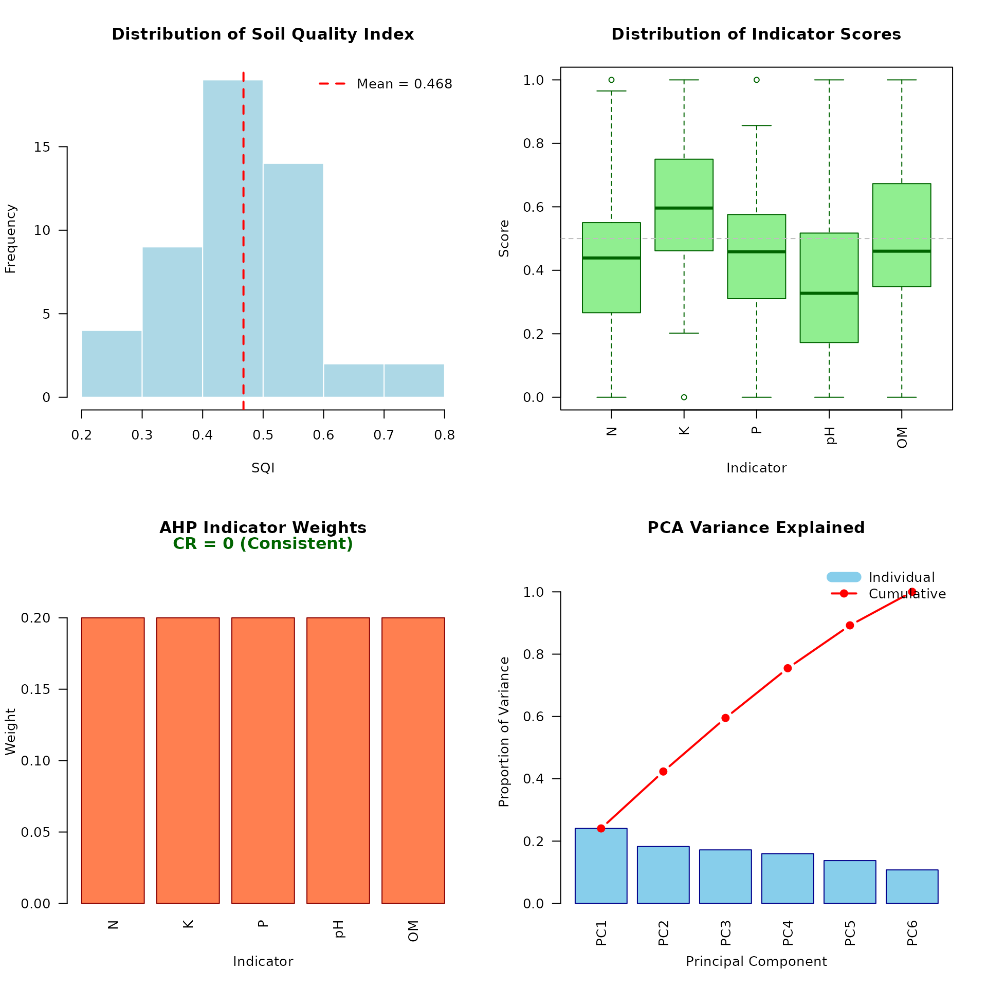
SQI Distribution

View the distribution of SQI values across all samples:

plot(result, type = "distribution")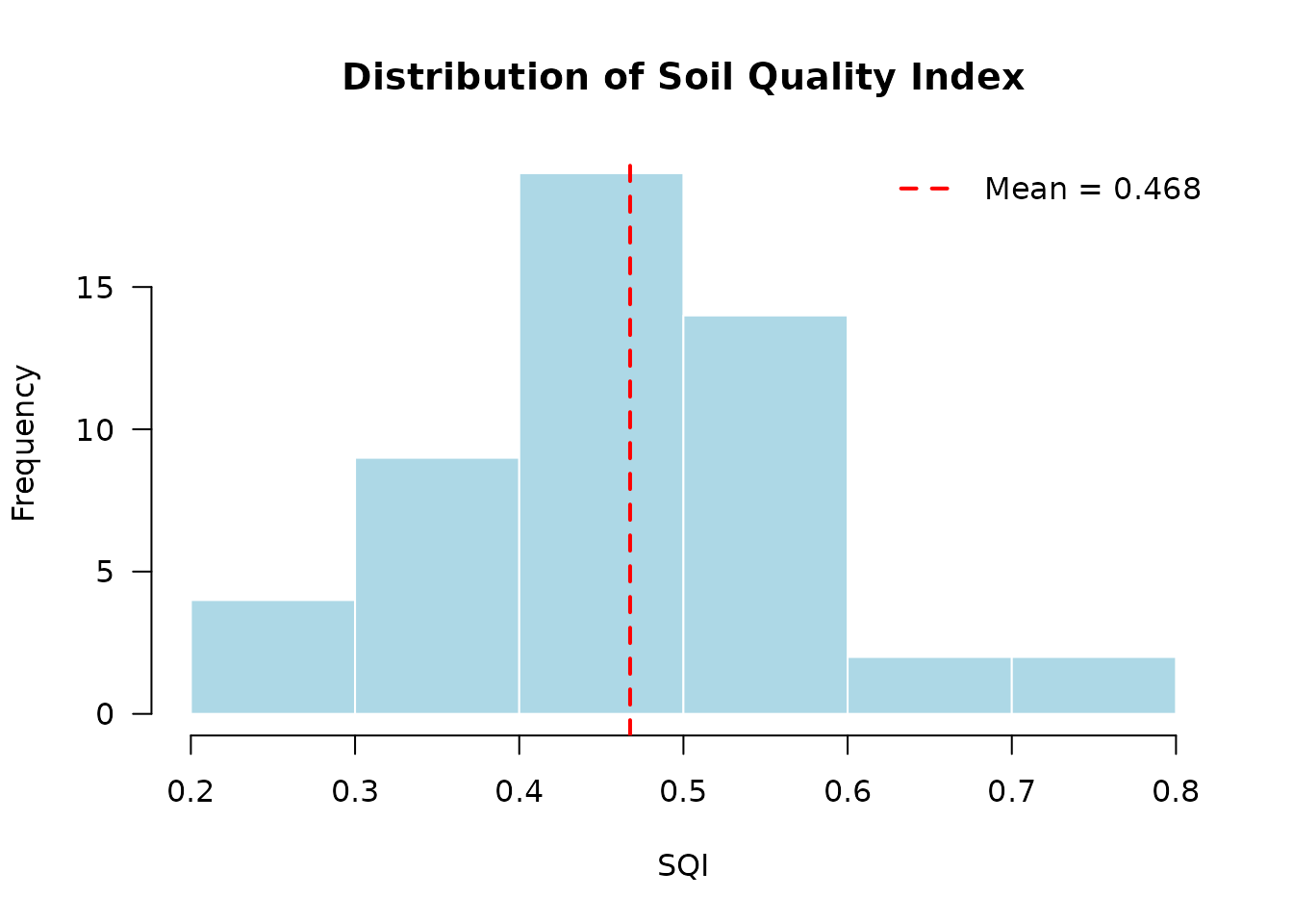

This histogram shows how SQI values are distributed, with a vertical line indicating the mean SQI.

Indicator Scores

Compare the scores of different indicators:

plot(result, type = "indicators")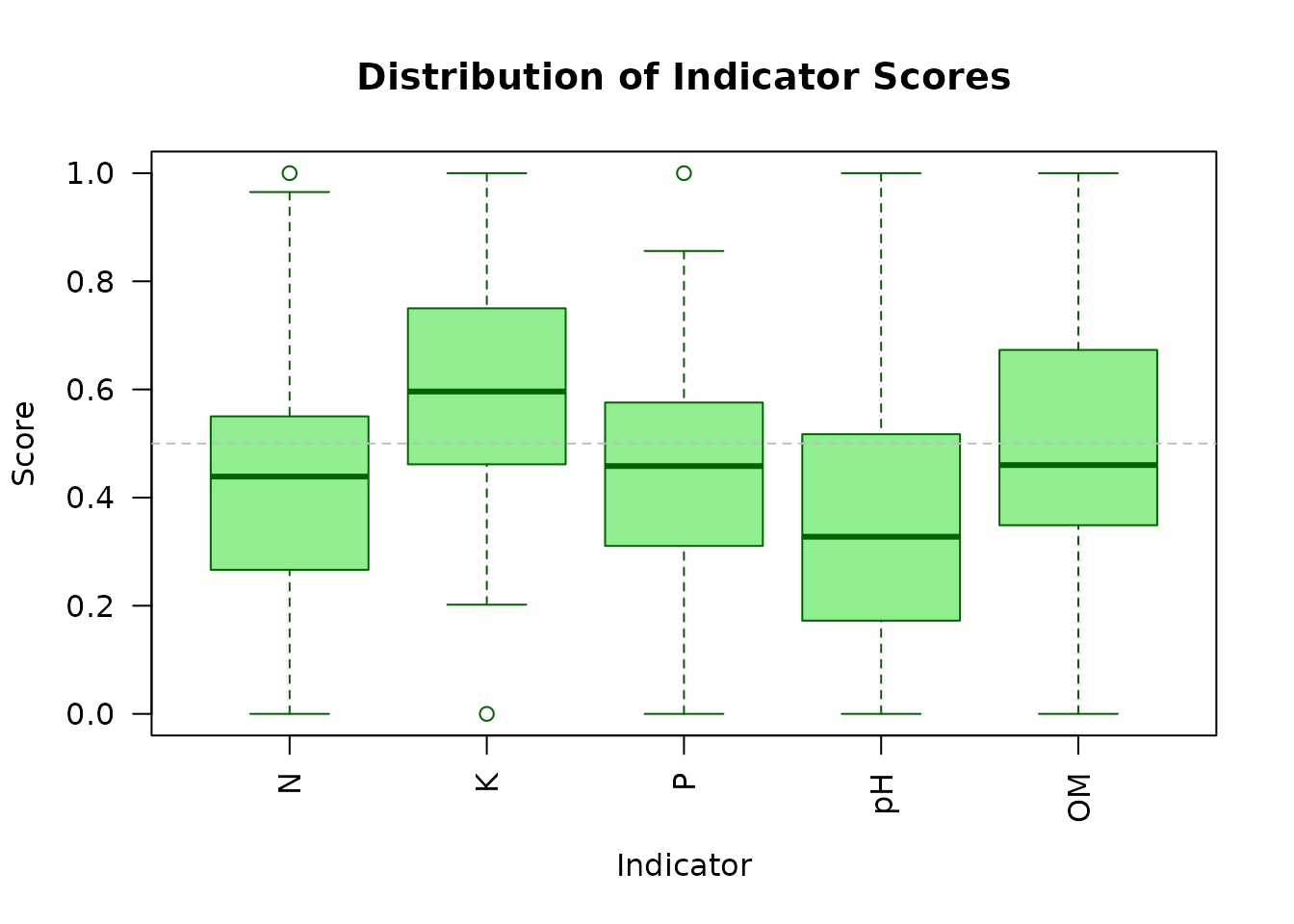

Boxplots show the distribution of scores for each MDS indicator, helping identify which properties are limiting soil quality.

Indicator Weights

View the relative importance of each indicator:

plot(result, type = "weights")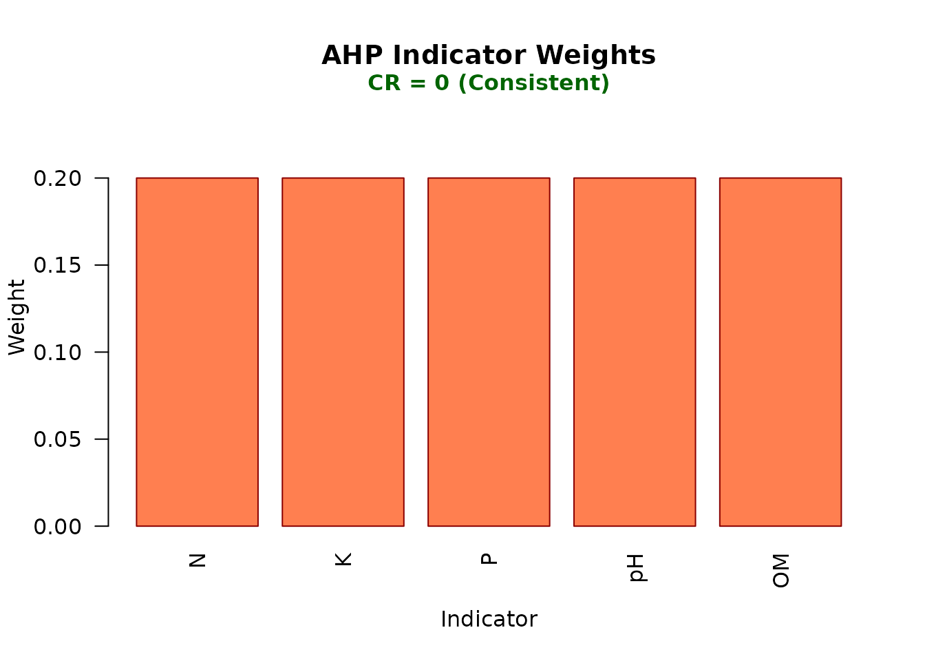

The bar chart shows the weight assigned to each indicator. The Consistency Ratio (CR) is displayed at the top.

PCA Scree Plot

Examine the variance explained by principal components:

plot(result, type = "scree")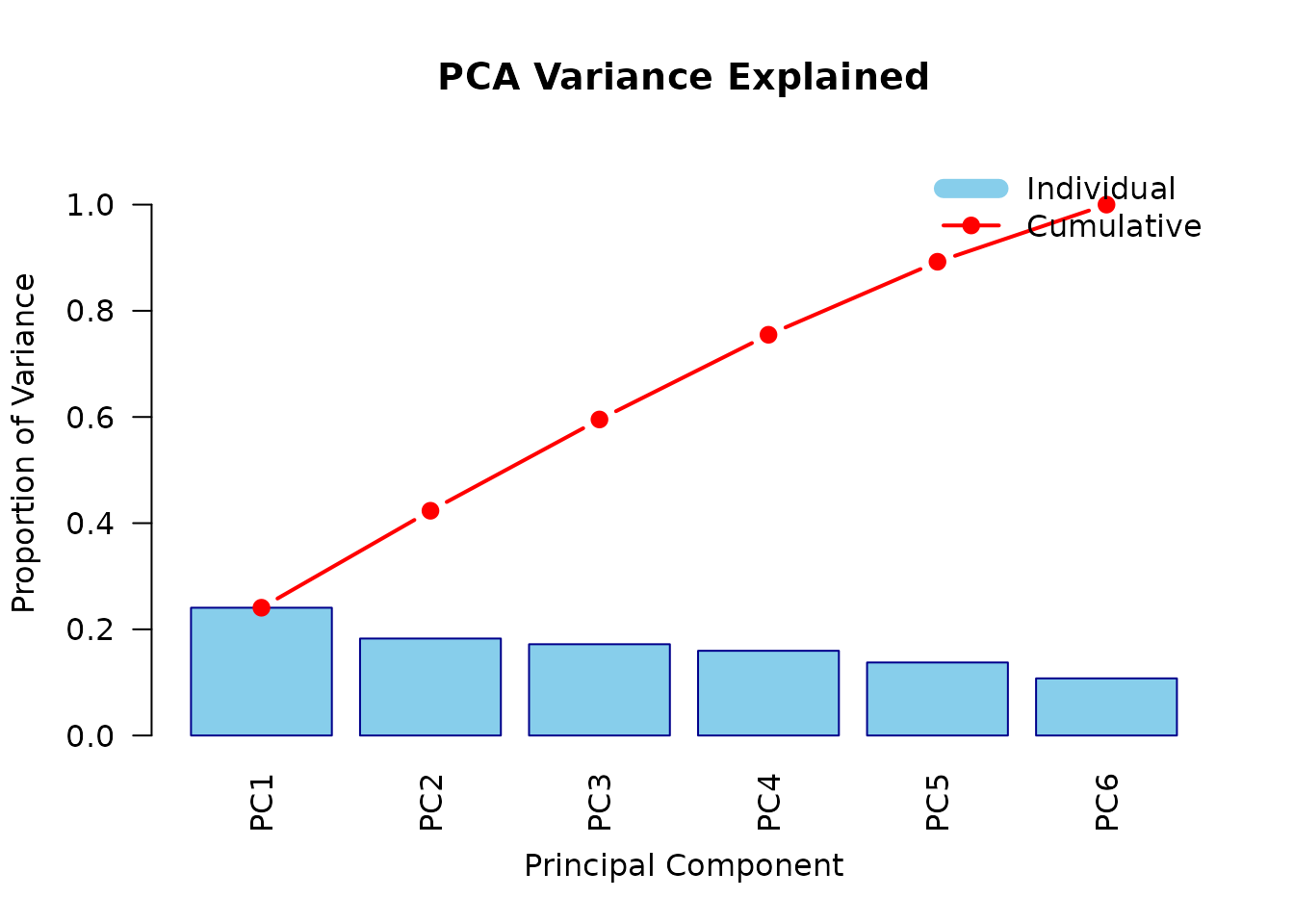

This plot helps understand how much variance is captured by the selected principal components.

Comprehensive Report

Generate all plots at once in a multi-panel layout:

plot_sqi_report(result)

Using Pre-defined Property Sets

The package includes several pre-defined property sets for common analyses:

# Available property sets
names(soil_property_sets)
#> [1] "basic"         "standard"      "comprehensive" "physical"     
#> [5] "chemical"      "fertility"

# View the standard property set
soil_property_sets$standard
#> [1] "Sand" "Silt" "Clay" "pH"   "OM"   "N"    "P"    "K"    "CEC"

# Use a pre-defined property set
result_standard <- compute_sqi_properties(
  data = soil_ucayali,
  properties = soil_property_sets$standard,
  id_column = "SampleID"
)

Available property sets:

basic: Essential properties (pH, OM, P, K)
standard: Common soil test properties
comprehensive: Extended property list
physical: Physical properties only
chemical: Chemical properties only
fertility: Fertility-related properties

Custom Property Selection

You can also specify your own custom set of properties:

# Focus on physical properties
physical_props <- c("Sand", "Silt", "Clay", "BD")

result_physical <- compute_sqi_properties(
  data = soil_ucayali,
  properties = physical_props,
  id_column = "SampleID"
)

# View selected MDS
result_physical$mds
#> [1] "Sand" "Clay" "BD"

Next Steps

This introduction covered the basic workflow for calculating SQI. To learn more:

Advanced Usage: See vignette("advanced-usage") for custom scoring rules, property selection strategies, and advanced visualization options
AHP Matrices: See vignette("ahp-matrices") for creating expert-based indicator weights using the Analytic Hierarchy Process
Function Reference: Use help(package = "soilquality") to browse all available functions

References

Andrews, S. S., Karlen, D. L., & Cambardella, C. A. (2004). The soil management assessment framework: A quantitative soil quality evaluation method. Soil Science Society of America Journal, 68(6), 1945-1962.
Saaty, T. L. (1980). The Analytic Hierarchy Process. McGraw-Hill.
Shukla, M. K., Lal, R., & Ebinger, M. (2006). Determining soil quality indicators by factor analysis. Soil and Tillage Research, 87(2), 194-204.

soilquality package

2025-12-26