Advanced Usage

soilquality package

2025-12-26

Introduction

This vignette covers advanced features of the soilquality package, including:

• Property selection strategies
• Custom scoring rules
• Creating and using AHP matrices
• Advanced visualization options
• Working with different data formats

library(soilquality)
data(soil_ucayali)

Property Selection Strategies

Choosing the right soil properties is crucial for meaningful SQI calculation. The package offers several approaches.

Strategy 1: Use Pre-defined Property Sets

The package includes curated property sets for common scenarios:

# View available property sets
names(soil_property_sets)
#> [1] "basic"         "standard"      "comprehensive" "physical"     
#> [5] "chemical"      "fertility"

# Compare different property sets
result_basic <- compute_sqi_properties(
  data = soil_ucayali,
  properties = soil_property_sets$basic,
  id_column = "SampleID"
)

# Use only fertility properties that exist in the dataset
fertility_available <- intersect(soil_property_sets$fertility, 
                                  names(soil_ucayali))
result_fertility <- compute_sqi_properties(
  data = soil_ucayali,
  properties = fertility_available,
  id_column = "SampleID"
)

# Compare mean SQI values
cat("Basic properties - Mean SQI:", 
    round(mean(result_basic$results$SQI), 3), "\n")
#> Basic properties - Mean SQI: 0.49
cat("Fertility properties - Mean SQI:", 
    round(mean(result_fertility$results$SQI), 3), "\n")
#> Fertility properties - Mean SQI: 0.508

Strategy 2: Domain-Specific Selection

Select properties based on your research question or management goal:

# For erosion risk assessment - focus on physical properties
erosion_props <- c("Sand", "Silt", "Clay", "BD", "OM")

result_erosion <- compute_sqi_properties(
  data = soil_ucayali,
  properties = erosion_props,
  id_column = "SampleID"
)

# For nutrient management - focus on fertility
nutrient_props <- c("pH", "OM", "N", "P", "K", "CEC")

result_nutrient <- compute_sqi_properties(
  data = soil_ucayali,
  properties = nutrient_props,
  id_column = "SampleID"
)

# Compare selected MDS
cat("Erosion assessment MDS:", paste(result_erosion$mds, collapse = ", "), "\n")
#> Erosion assessment MDS: Sand, Clay, BD, OM
cat("Nutrient management MDS:", paste(result_nutrient$mds, collapse = ", "), "\n")
#> Nutrient management MDS: N, K, P, pH, OM

Strategy 3: Data-Driven Selection

Let PCA automatically select the most informative properties:

# Use all available numeric properties
all_numeric <- names(soil_ucayali)[sapply(soil_ucayali, is.numeric)]

result_all <- compute_sqi_properties(
  data = soil_ucayali,
  properties = all_numeric,
  id_column = "SampleID"
)

# See which properties were selected by PCA
cat("PCA selected:", length(result_all$mds), "indicators from", 
    length(all_numeric), "properties\n")
#> PCA selected: 8 indicators from 14 properties
print(result_all$mds)
#> [1] "Sand" "Silt" "Ca"   "SOC"  "OM"   "pH"   "Mg"   "P"

Strategy 4: Correlation-Based Pre-screening

Remove highly correlated properties before analysis:

# Calculate correlation matrix
numeric_data <- soil_ucayali[, sapply(soil_ucayali, is.numeric)]
cor_matrix <- cor(numeric_data, use = "complete.obs")

# Find highly correlated pairs (|r| > 0.9)
high_cor <- which(abs(cor_matrix) > 0.9 & cor_matrix < 1, arr.ind = TRUE)

if (nrow(high_cor) > 0) {
  cat("Highly correlated property pairs:\n")
  for (i in 1:nrow(high_cor)) {
    if (high_cor[i, 1] < high_cor[i, 2]) {  # Avoid duplicates
      cat(sprintf("  %s - %s: r = %.3f\n",
                  rownames(cor_matrix)[high_cor[i, 1]],
                  colnames(cor_matrix)[high_cor[i, 2]],
                  cor_matrix[high_cor[i, 1], high_cor[i, 2]]))
    }
  }
}

# Remove one from each highly correlated pair
# For example, keep SOC but remove OM (they're highly correlated)
reduced_props <- setdiff(all_numeric, c("OM"))

result_reduced <- compute_sqi_properties(
  data = soil_ucayali,
  properties = reduced_props,
  id_column = "SampleID"
)

Custom Scoring Rules

The package provides flexible scoring functions to match different soil property behaviors.

Higher is Better

For properties where higher values indicate better soil quality:

# Organic matter, nutrients, CEC
scoring_rules <- list(
  OM = higher_better(),
  N = higher_better(),
  P = higher_better(),
  K = higher_better(),
  CEC = higher_better()
)

result_higher <- compute_sqi_properties(
  data = soil_ucayali,
  properties = names(scoring_rules),
  scoring_rules = scoring_rules,
  id_column = "SampleID"
)

Lower is Better

For properties where lower values indicate better soil quality:

# Bulk density, electrical conductivity
scoring_rules_lower <- list(
  BD = lower_better(),
  EC = lower_better()
)

result_lower <- compute_sqi_properties(
  data = soil_ucayali,
  properties = names(scoring_rules_lower),
  scoring_rules = scoring_rules_lower,
  id_column = "SampleID"
)

Optimum Range

For properties with an ideal target value:

# pH has an optimal range around neutral
scoring_rules_opt <- list(
  pH = optimum_range(optimal = 6.5, tolerance = 1.5),
  Sand = higher_better(),
  Clay = higher_better(),
  OM = higher_better()
)

result_opt <- compute_sqi_properties(
  data = soil_ucayali,
  properties = names(scoring_rules_opt),
  scoring_rules = scoring_rules_opt,
  id_column = "SampleID"
)

# Compare pH scoring with different optimal values
result_opt_7 <- compute_sqi_properties(
  data = soil_ucayali,
  properties = c("pH", "OM", "N", "P"),
  scoring_rules = list(
    pH = optimum_range(optimal = 7.0, tolerance = 1.0),
    OM = higher_better(),
    N = higher_better(),
    P = higher_better()
  ),
  id_column = "SampleID"
)

cat("Mean SQI with pH optimum 6.5:", 
    round(mean(result_opt$results$SQI), 3), "\n")
#> Mean SQI with pH optimum 6.5: 0.395
cat("Mean SQI with pH optimum 7.0:", 
    round(mean(result_opt_7$results$SQI), 3), "\n")
#> Mean SQI with pH optimum 7.0: 0.336

Threshold-Based Scoring

For properties with specific threshold values:

# Example: P availability with agronomic thresholds
# Low: <10, Medium: 10-20, High: 20-40, Very High: >40
scoring_rules_thresh <- list(
  P = threshold_scoring(
    thresholds = c(0, 10, 20, 40, 100),
    scores = c(0, 0.4, 0.7, 1.0, 1.0)
  ),
  K = threshold_scoring(
    thresholds = c(0, 50, 100, 200, 500),
    scores = c(0, 0.4, 0.7, 1.0, 1.0)
  ),
  OM = higher_better(),
  pH = optimum_range(optimal = 6.5, tolerance = 1.5)
)

result_thresh <- compute_sqi_properties(
  data = soil_ucayali,
  properties = names(scoring_rules_thresh),
  scoring_rules = scoring_rules_thresh,
  id_column = "SampleID"
)

Mixed Scoring Strategies

Combine different scoring approaches for comprehensive assessment:

# Realistic scoring for tropical agricultural soils
tropical_scoring <- list(
  pH = optimum_range(optimal = 6.0, tolerance = 1.5),
  OM = higher_better(),
  SOC = higher_better(),
  N = higher_better(),
  P = threshold_scoring(
    thresholds = c(0, 8, 15, 30, 100),
    scores = c(0.2, 0.5, 0.8, 1.0, 1.0)
  ),
  K = threshold_scoring(
    thresholds = c(0, 60, 120, 200, 500),
    scores = c(0.2, 0.5, 0.8, 1.0, 1.0)
  ),
  CEC = higher_better(),
  BD = lower_better(),
  EC = lower_better()
)

result_tropical <- compute_sqi_properties(
  data = soil_ucayali,
  properties = names(tropical_scoring),
  scoring_rules = tropical_scoring,
  id_column = "SampleID"
)

cat("Tropical scoring - Mean SQI:", 
    round(mean(result_tropical$results$SQI), 3), "\n")
#> Tropical scoring - Mean SQI: 0.493

Creating AHP Matrices

The Analytic Hierarchy Process (AHP) allows expert-based weighting of indicators.

Method 1: Interactive Creation

Create a pairwise comparison matrix interactively:

# This will prompt you for pairwise comparisons
indicators <- c("pH", "OM", "P", "K")
ahp_matrix <- create_ahp_matrix(indicators, mode = "interactive")

# Use the AHP matrix in SQI calculation
result_ahp <- compute_sqi_properties(
  data = soil_ucayali,
  properties = indicators,
  pairwise_matrix = ahp_matrix$matrix,
  id_column = "SampleID"
)

Method 2: Manual Matrix Creation

Create a pairwise comparison matrix manually:

# Define indicators
indicators <- c("pH", "OM", "N", "P")

# Create pairwise comparison matrix
# Rows are compared to columns
# Values: 1=Equal, 3=Moderate, 5=Strong, 7=Very Strong, 9=Extreme
pairwise <- matrix(c(
  1,   1/3, 1/5, 1/3,  # pH compared to others
  3,   1,   1/3, 1,    # OM compared to others
  5,   3,   1,   3,    # N compared to others
  3,   1,   1/3, 1     # P compared to others
), nrow = 4, byrow = TRUE)

colnames(pairwise) <- rownames(pairwise) <- indicators

# Calculate weights
ahp_result <- ahp_weights(pairwise, indicators = indicators)

cat("Indicator weights:\n")
#> Indicator weights:
print(round(ahp_result$weights, 3))
#>    pH    OM     N     P 
#> 0.078 0.200 0.522 0.200
cat("\nConsistency Ratio:", round(ahp_result$CR, 4), "\n")
#> 
#> Consistency Ratio: 0.0161

# Note: To use AHP weights in SQI calculation, the pairwise matrix must match
# the MDS indicators selected by PCA. For this example, we'll calculate SQI
# with equal weights and show the AHP weights separately.
result_manual_ahp <- compute_sqi_properties(
  data = soil_ucayali,
  properties = indicators,
  id_column = "SampleID"
)

cat("\nMDS indicators selected by PCA:", paste(result_manual_ahp$mds, collapse = ", "), "\n")
#> 
#> MDS indicators selected by PCA: N, pH, OM

Method 3: Importance Ratios

Use relative importance ratios (simpler than full pairwise matrix):

# Specify relative importance (e.g., N is 3x more important than pH)
indicators <- c("pH", "OM", "N", "P")
importance_ratios <- c(1, 2, 3, 2)  # Relative importance

# Convert to pairwise matrix
pairwise_from_ratios <- ratio_to_saaty(importance_ratios)
colnames(pairwise_from_ratios) <- rownames(pairwise_from_ratios) <- indicators

# Calculate weights
ahp_from_ratios <- ahp_weights(pairwise_from_ratios, indicators = indicators)

cat("Weights from importance ratios:\n")
#> Weights from importance ratios:
print(round(ahp_from_ratios$weights, 3))
#>    pH    OM     N     P 
#> 0.125 0.250 0.375 0.250

Advanced Visualization

Customizing Plot Appearance

# Calculate SQI for visualization examples
result_viz <- compute_sqi_properties(
  data = soil_ucayali,
  properties = c("pH", "OM", "N", "P", "K", "CEC"),
  id_column = "SampleID"
)

# Distribution plot
plot(result_viz, type = "distribution")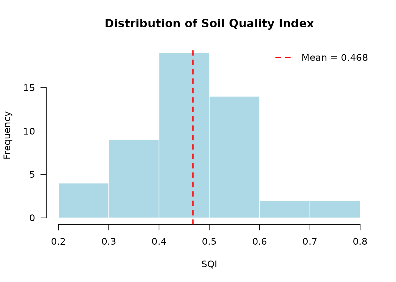

Comparing Multiple Scenarios

# Calculate SQI with different property sets
result_physical <- compute_sqi_properties(
  data = soil_ucayali,
  properties = soil_property_sets$physical,
  id_column = "SampleID"
)

# Use only chemical properties that exist in the dataset
chemical_available <- intersect(soil_property_sets$chemical, 
                                 names(soil_ucayali))
result_chemical <- compute_sqi_properties(
  data = soil_ucayali,
  properties = chemical_available,
  id_column = "SampleID"
)

# Compare distributions
par(mfrow = c(1, 2))
hist(result_physical$results$SQI, 
     main = "Physical Properties",
     xlab = "SQI", col = "lightblue", xlim = c(0, 1))
abline(v = mean(result_physical$results$SQI), col = "red", lwd = 2)

hist(result_chemical$results$SQI, 
     main = "Chemical Properties",
     xlab = "SQI", col = "lightgreen", xlim = c(0, 1))
abline(v = mean(result_chemical$results$SQI), col = "red", lwd = 2)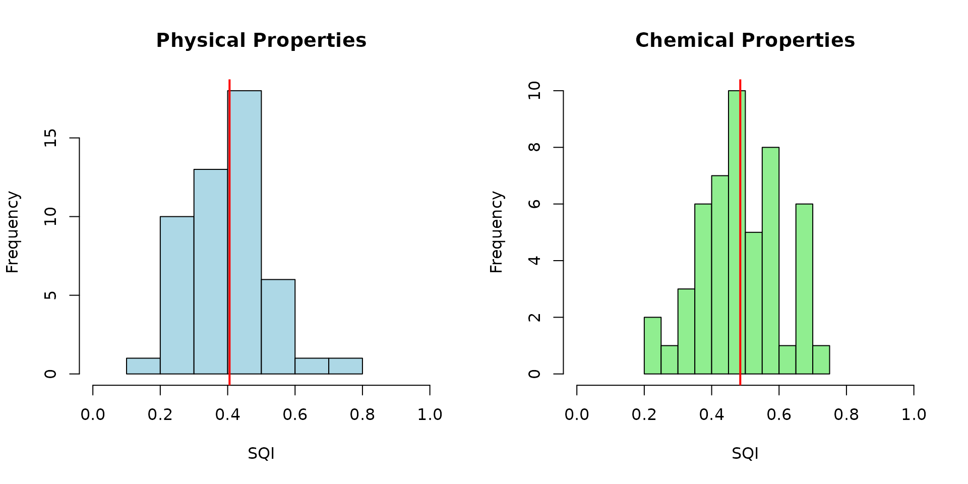

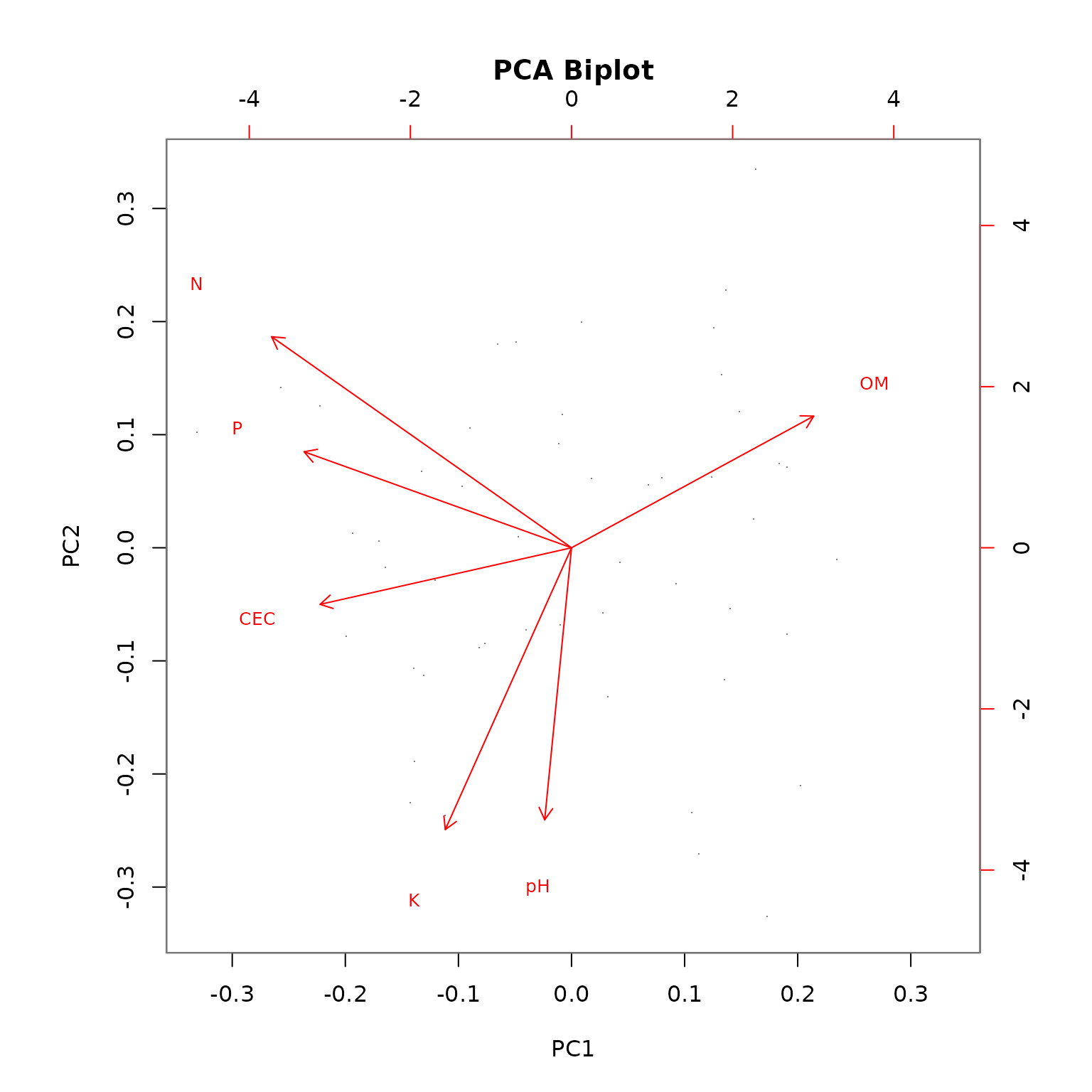
par(mfrow = c(1, 1))

PCA Biplot

Visualize relationships between samples and variables:

plot(result_viz, type = "biplot")

Indicator Contribution Analysis

Identify which indicators contribute most to SQI variation:

# Extract scored indicators and weights
scored_data <- result_viz$results[, paste0(result_viz$mds, "_scored")]
weights <- result_viz$weights

# Calculate weighted contribution of each indicator
contributions <- sweep(scored_data, 2, weights, "*")

# Plot contributions
boxplot(contributions, 
        main = "Weighted Indicator Contributions to SQI",
        ylab = "Weighted Score",
        las = 2,
        col = rainbow(length(result_viz$mds)))

Working with Different Data Formats

File-Based Workflow

# Save data to CSV
write.csv(soil_ucayali, "soil_data.csv", row.names = FALSE)

# Calculate SQI from file
result_from_file <- compute_sqi(
  input_csv = "soil_data.csv",
  id_column = "SampleID",
  output_csv = "sqi_results.csv"
)

# Results are automatically saved to output_csv

Data Frame Workflow

# Work directly with data frames (no file I/O)
result_df <- compute_sqi_df(
  df = soil_ucayali,
  id_column = "SampleID"
)

# Extract results
sqi_values <- result_df$results$SQI
names(sqi_values) <- result_df$results$SampleID

# View top 5 samples by SQI
head(sort(sqi_values, decreasing = TRUE), 5)
#>    UCY043    UCY005    UCY001    UCY050    UCY045 
#> 0.6927483 0.6061193 0.5852834 0.5773329 0.5691887

Batch Processing Multiple Datasets

# Process multiple sites or time points
sites <- c("site1.csv", "site2.csv", "site3.csv")

results_list <- lapply(sites, function(site) {
  compute_sqi(
    input_csv = site,
    id_column = "SampleID",
    properties = soil_property_sets$standard
  )
})

# Compare mean SQI across sites
mean_sqi <- sapply(results_list, function(r) mean(r$results$SQI))
names(mean_sqi) <- sites
print(mean_sqi)

Best Practices

1. Property Selection

• Use at least 5-6 properties for robust PCA
• Include properties from different categories (physical, chemical, biological)
• Avoid highly correlated properties (|r| > 0.9)
• Match properties to your management objectives

2. Scoring Rules

• Use domain knowledge to select appropriate scoring functions
• Validate scoring rules with local experts or literature
• Consider regional differences in optimal values
• Document your scoring rationale

3. AHP Weighting

• Involve multiple experts for more reliable weights
• Check Consistency Ratio (CR < 0.1)
• Use equal weights if expert knowledge is unavailable
• Sensitivity analysis: test how results change with different weights

4. Interpretation

• Consider SQI in context of land use and management goals
• Compare SQI across similar soil types or land uses
• Use visualization to identify limiting factors
• Validate results with field observations

Summary

This vignette demonstrated advanced features including:

• Multiple property selection strategies
• Custom scoring rules for different property behaviors
• Creating AHP matrices for expert-based weighting
• Advanced visualization and comparison techniques
• Different data workflow options

For more information on AHP methodology, see vignette("ahp-matrices").

References

• Karlen, D. L., Mausbach, M. J., Doran, J. W., Cline, R. G., Harris, R. F., & Schuman, G. E. (1997). Soil quality: A concept, definition, and framework for evaluation. Soil Science Society of America Journal, 61(1), 4-10.

• Qi, Y., Darilek, J. L., Huang, B., Zhao, Y., Sun, W., & Gu, Z. (2009). Evaluating soil quality indices in an agricultural region of Jiangsu Province, China. Geoderma, 149(3-4), 325-334.